The Energy Balance Model
Of Physics and Politics
My previous post, The True Nature of the Climate Crisis, covered the scope of the problem and provided an initial sketch of solution options. It ended with Professor Kevin Anderson’s observation that there are no more non-radical futures left. Anderson is extremely clear that irrespective of what politicians, business people or technologists say or believe, there is no dematerial deal of any flavour (new, green or artful) that can be made with nature. The Real has the final say and is increasingly making its voice heard everywhere. Artificial Intelligence cannot help us escape the noumenal realm unless it is given agency by us to apply Physics:
In this post we’re going to dive quite a bit deeper into the Energy Balance Model or EBM introduced in the first post. The EBM is the foundation for all climate modelling. Learning how an EBM works is an essential first step in demystifying climate science and climate literacy. Knowing about the different EBM elements and the way they interact with one another furnishes you with an intuitive understanding of the Physics behind climate change. Having said that, it is important to remember that a model is a tool for exploring reality and all models have to make assumptions and simplifications in their construction. I’ll go into a fair bit of detail on the EBM because I think it matters given what is at stake.
The concepts involved are reasonably straightforward especially for the most basic form of EBM. The maths becomes more complex involving linear equations as we start adding atmospheric effects. There are three key features to consider in the EBM:
Solar flux. Radiation from the sun in the visible part of the spectrum landing on earth.
Albedo effect. Albedo is the fraction of sunlight that is diffusely reflected by a body. Around 30% of solar flux is reflected by ice caps and clouds.
Energy balance. For equilibrium, the energy into the earth system equals energy out.
Any mismatch between energy entering the earth system as solar flux and energy escaping it as long wave radiation drives temperature change. Now let’s look at each of these three features in turn.
1. Solar flux
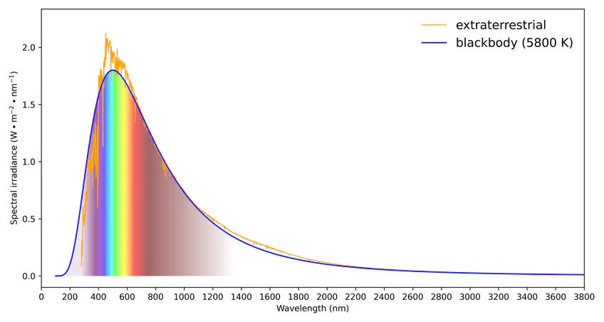
The sun is a free energy source that we can model as a black body. This is an object that absorbs and emits electromagnetic radiation in accordance with the thermal motion of its particles. The spectrum of this radiation depends on its temperature. We can use Planck’s Law to model the sun’s radiation using a surface temperature of 5800K. We can then compare that model with actual measured radiation which we observe covers the entire spectrum from gamma rays to radio waves. Radiation peaks in the visible light region which is why the sun appears white in space. Modelled and measured spectra are closely correlated as illustrated below:
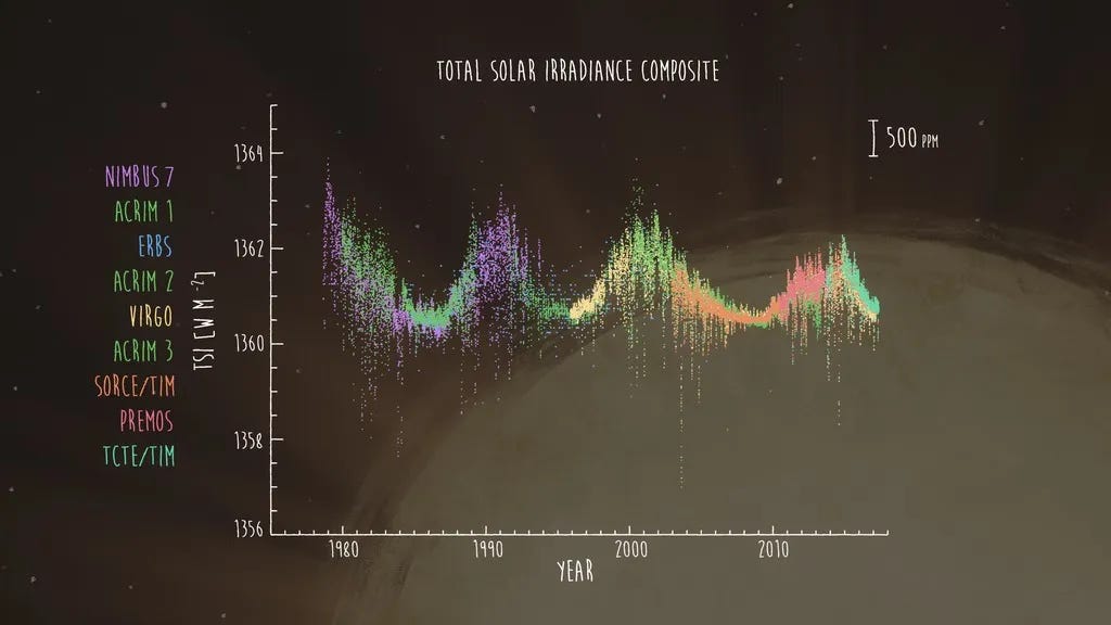
Solar irradiance is the power per unit area of solar flux. It is measured in watts per square metre (W/m2). Total solar irradiance or TSI is a measure of this solar flux integrated over all wavelengths per unit area incident on earth’s upper atmosphere measured perpendicular to incoming sunlight. An Astronomical Unit (AU) is the average distance between the earth and the sun. The average measure for TSI at one AU is referred to as the solar constant (S) which is 1366 W/m2. The “constant” here is a misnomer because TSI does vary but very slowly and typically on long cycles. It will only change significantly and increase by 10% over a billion years. The solar cycle is one such periodic variation of TSI. It lasts around 11 years with a peak characterised by a high number of sunspots and the flipping of the sun’s magnetic poles. Our next peak is due in 2025. It’s possible to see this solar cycle in action by examining measurements from satellite data. The NASA graphic below shows a composite of TSI measurements from nine satellites launched since 1978. Note from the y-axis that the absolute variation of the solar cycle is really small - of the order of 0.1% between peak and trough:
NASA also provides TSI data from the Total and Spectral solar Irradiance Sensor (TSIS-1), a probe on the International Space Station (ISS) that was launched by NASA in late 2017 to measure TSI. The graph below is from an accompanying notebook that details how to download and graph this data using Python. It shows our approach towards a local maximum.
Solar flux on earth is determined by its cross section or πRE2 where RE is the earth’s radius. As earth rotates, this energy is distributed across the entire surface area 4πRE2 so the average incoming solar flux the earth receives is ¼ the solar constant or S/4 which is around 340W/m2.
2. Albedo Effect
Not all solar flux arriving at the top of the atmosphere or TOA, as climate scientists refer to it, makes it to the surface of the earth. The TOA is approximately 100 km up from the surface. Around 30% of radiation at TOA is reflected back by clouds and by various surfaces encountered including ice before it reaches the ground. The albedo of different materials vary as the table below illustrates. Substances such as snow and ice are highly reflective. Water, forests and roads much less so. Note how losing super reflective ice caps on land reduces the albedo of that land mass significantly from around 0.7 to 0.2 further compounding warming:
We can model average albedo for earth using a parameter α which is around 0.3. Removing the reflected flux from that at TOA we therefore arrive at the following estimate for the average solar flux which makes it to the ground to be absorbed by earth: (1-α)S/4 W/m2. This is widely known as the absorbed shortwave radiation or ASR.
3. Energy Balance
ASR absorbed by the earth is re-radiated back out into space as infrared or longwave radiation. We can model this longwave radiation by considering the earth to be a black body and using the Stefan-Boltzmann law. This law is derived from Planck’s Law and describes the thermal radiation emitted by matter purely in terms of that matter’s temperature. The Stefan–Boltzmann law states that the total power radiated per unit surface area is equal to the fourth power of the black body's temperature, T, multiplied by the Stefan-Boltzmann constant σ. In other words, σT4 W/m2. The proportion of this ASR that makes it back out into space is called the outgoing longwave radiation or OLR.
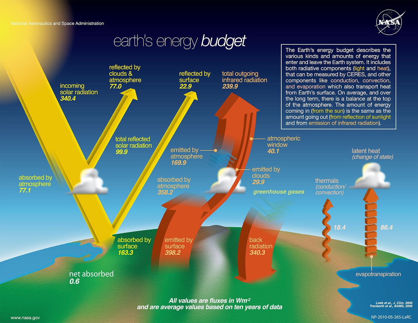
The NASA diagram below from their resource page on earth’s Energy Budget shows incoming solar flux at TOA, the total proportions reflected by clouds and the surface of earth, the corresponding ASR absorbed by earth and the total proportion that makes it out into space as OLR.
The foundational principle of all EBMs is that ASR=OLR thus yielding an equilibrium temperature T. We can therefore construct our first and simplest thermodynamic energy balance model if we assume in the first instance that all the ASR makes it back out into space at TOA. If we set ASR = OLR we get the following equation:
(1-α)S/4 = σT4
We can solve for T in this equation using values of α=0.30, S=1372 W/m2, Q=S/4 and σ= 5.67x10⁻⁸ W/m2K4 as shown in the outline below from another accompanying notebook that works through the EBM from first principles using Python. The resulting temperature of 255K or -18C is much colder than we observe because not the assumption that 100% of ASR makes it back out to space is not valid. A proportion is absorbed by greenhouse gases in the atmosphere and stays in the earth system resulting in atmospheric warming. This energy is vital for maintaining life on earth and driving weather systems. It helped produce a Goldilocks climate that supported the rise of Agriculture.
We can model the scale of the greenhouse effect with an emissivity factor ε that accounts for the earth not being a perfect black body radiator on account of the atmosphere. A value of 0.61 for ε yields the measured average earth surface temperature of 288.65K. Surface temperature remained close to this value for twelve thousand years prior to the Industrial Revolution during which we were in thermal equilibrium with energy in and energy out being balanced:
Over the last 250 years, human activities have resulted in the emission of large quantities of greenhouse gases that natural carbon sinks have not been able to absorb, disturbing the equilibrium. These activities have produced radiative forcing driving additional atmospheric warming due to the mismatch between incoming solar radiation and the proportion absorbed by the atmosphere. In essence our emissivity factor ε has decreased, pushing earth’s radiative balance away from its pre-industrial state towards a higher temperature.
Refined EBM models
Thus far, we have worked with the simplest possible EBM with an emissivity factor as a master dial to get us to the right result we observe. Can we improve upon that with a refined model? Yes, we can. We start by introducing the earth’s atmosphere as a single layer in the model with equal downwelling and upwelling radiation components as illustrated below from the same EBM notebook. We employ this approach because Kirchhoff’s Law states that the radiation absorbed at any atmospheric layer is emitted equally upward and downward. EBMs that employ this principle are known as grey gas models. The corresponding updated radiative transfer equations now yield a revised equilibrium temperature of 303 K, which is approximately 30 °C too high.
There are further refinements that can be made. The atmosphere is not a uniform single layer. We can simulate the troposphere and stratosphere in a two layer grey gas model with a dividing line at 500 hPa pressure level which is approximately 5.5km up from sea level. This gets us to 296K which is 8C higher than our desired target of 288K. Incorporating two layers requires us to start working with matrices and solve linear equations for the temperature at the top of each layer. We can manage that by hand as illustrated in the EBM notebook. We can go further and create a 30 layer grey gas model. It gets very onerous to calculate the equations for that without help so the notebooks uses an open source climate modelling package called climlab to model the behaviour of convection and the impact of ozone in the upper atmosphere. Doing so gets us very much closer to observed temperature values though the atmosphere which is known as the lapse rate. It is important to model lapse rate accurately because it is non-linear. We do not observe a continuous drop in temperature going up through the stratosphere. We see more of a U-shape.
Two of the key predictions of early climate models were the exaggeration of these twin phenomena of tropospheric warming and stratospheric cooling as CO2 concentrations increased. In other words, they predicted that we would observe warmer temperatures at the surface and counterintuitively cooler temperatures in the upper atmosphere as GHG emissions rose. The reasons why are beyond our scope here but the data is covered in a bit more detail in the EBM notebook and this video attempts to explain what is going on in terms of the Physics of infrared radiation and absorption:
Stratospheric cooling in particular is the smoking gun that pins climate change to GHG emissions.
Adding more atmospheric layers also helps us model convective warming which is the mechanism that is warming the Arctic faster than the rest of the world:
additional warming caused by carbon dioxide and other greenhouse gases mainly affects the atmosphere near the surface. In the tropics, this extra warmth gets spread vertically due to convection. But in the Arctic, the warming from greenhouse gases is most pronounced near the surface.
Going beyond the EBM requires us to take into account human impacts which haven’t been factored in yet. A number of approaches have been developed over the last few decades which has resulted in a taxonomy of models. Here’s a brief outline of some of the most important categories being used today by IPCC scientists to predict climate change and project future greenhouse gas concentrations:
Radiative-Convective (RC) or Single-Column Models (SCMs): These models focus on processes in the vertical air column. RC models compute the (usually global average) temperature profile by explicit modelling of radiation and convection processes to more accurately predict the measured lapse rate.
Integrated Assessment Models (IAMs): These models directly factor in economic activity within modelling to more fully assess the impact of particular policy choices affective emissions. They are able to factor in human development and societal choices and are particularly useful for climate mitigation purposes. The most notable examples are the IPCC Representative Concentration Pathways (RCPs). The model used in the En-ROADS climate simulator introduced in the previous post is a form of IAM. See here for more context.
Global Circulation Models (GCMs): These Physics-based models simulate the full, three-dimensional energy dynamics of the atmosphere and ocean. They can exist as fully coupled ocean-atmosphere models or as independent ocean or atmospheric circulation models. By simulating all large-scale climate processes, they can produce a three-dimensional picture of the time evolution of the state of the whole climate system. GCMs are able to make climate predictions through time-stepping but their accuracy is limited by the scale of computer power made available to them. Earlier this year Google released their Neural GCM which uses neural networks to further improve the accuracy of GCM predictions by using ML techniques to enable the modelling of smaller scale phenomena.. These show promise in more accurately forecasting climate processes such cloud formation and precipitation. Google highlighted that this approach “generates 2–15 day weather forecasts that are more accurate than the current gold-standard physics-based model, and reproduces temperatures over a past 40-year period more accurately than traditional atmospheric models.”
Earth System Models (ESMs): Moving further forward in climate modelling history, additional processes that used to be fixed come to be incorporated into GCMs and the coupling becomes more complete including changes in biomes and vegetation, chemical changes in atmosphere, ocean and soil as well as anthropogenic impacts. Such models are now generally known as Earth System Models. CESM is a community effort to build an ESM.
This is a good point to pause and take stock. We have taken quite a ride through the Energy Balance Model including various progressive refinements to more closely model what we observe. The goal was to provide you with a basic understanding from first principles of some of the Physics behind climate modelling. If you’ve followed along, you should hopefully have developed more insight into climate science. Current models are far more sophisticated and more accurate than the EBM but even so, several aspects remain that need further improvement such as:
Climate sensibility, specifically the Equilibrium Climate Sensitivity (ECS) which is a measure of how much warming occurs after we double atmospheric CO2 concentration. Current estimates range from about 1.5C to 4.5C.
Carbon sink and source performance in response to further warming. Permafrost thawing potential for instance.
Cloud formation, development and feedback effects particularly in relation to interaction with aerosols.
Ocean processes such as the Atlantic Meridional Overturning Circulation (AMOC) which gives rise to the Gulf Stream.
Ice sheet melt particularly in Antarctica and the corresponding impact in terms of sea level rise.
Tipping points and non-linear responses driven by positive feedback. For example the recent prediction of wind speed reduction.
Locally specific extreme weather event prediction.
Climate models provide a compass for corresponding solutions which in turn are meant to drive political action. We saw in the previous post how we can model the impact of that action in the En-ROADS simulator. The international political system based around yearly COP events feels increasingly incapable of keeping pace with what we are learning about the growing urgency of our current climate situation. As little as a decade ago, we thought we had a lot longer to avert the worst case scenarios. Now the evidence suggests we will hit multiple tipping points with just 1.5C-2C rise which is more or less a given. As the severity of climate change impacts grow globally over the coming decade, it seems likely that radical short term crash interventions to manipulate solar flux will gather increasing support in parallel. In particular solar radiation management (SRM) methods which are considered unacceptable by many today. Next time in the series we’ll consider this broader mitigation landscape and dive deeper on SRM.


